 project. The work has been during the spring semester, and
is stipulated to 20 hours of work per week per person, giving a total
of 520 hours.
Torgeir Dingsřyr - Endre M. Lidal
Three methods for Data Mining were discussed for use in cooperation with Case-Based Reasoning: Bayesian Networks, Inductive Logic Programming and Rough Sets. Experiments were carried out on AutoClass, which is a Bayesian classifier, and on Rosetta, which is a Rough Set tool producing logic rules. The dataset used for the experiments were taken from a reliability database for the oil industry, OREDA. The Rough Set method produces many rules, and the overfit increases with the size of the training set. Bayesian classification can reveal poor human classification in the dataset, but requires much human interpretation of the result. The rule generated from Rosetta can be used as background knowledge in Case-Based Reasoning, and in making predictions about failures.
This report is written as a project in Course 45073 Computer Science
Projects at the Department of Computer and Information
Science at the Norwegian University of Science and Technology in
Trondheim. It is a part of the NOEMIE project. The work has been during the spring semester, and
is stipulated to 20 hours of work per week per person, giving a total
of 520 hours.
Through the work with this project, we have had many useful of discussions with people from the Department of Computer and Information Science.
We would like to thank Alexander Řhrn for help with Rosetta, Torulf Mollestad for explaining properties of Rough Sets. Řystein Nytrř and Erling Alfheim for discussions on Inductive Logic Programming, and Knut Magne Risvik for discussions on Data Mining in general.
We would also like to thank John Stutz and Will Taylor at NASA Ames Research Center for answering questions about AutoClass. Knut Haugen at SINTEF helped us gain an understanding of the OREDA database.
Through the work on the project, we have followed lectures in Computer Intensive Statistics and Logics for Computer Science. Through the last course we have been able to discuss many of the problems we have met in experimenting with the data.
Finally, we would like to thank our supervisors, professor Agnar Aamodt and professor Jan Komorowski at the Department of Computer and Information Science, NTNU, and Ole Martin Winnem at SINTEF.
Trondheim, 29th of April, 1997,
¯Endre Mřlster Lidal Torgeir Dingsřyr
The purpose of this report is to evaluate methods and tools for Knowledge Discovery and Data Mining, in the context of integrating Case Based Reasoning and Data Mining techniques. We have chosen the methods Bayesian Networks, Inductive Logic Programming and Rough Sets for evaluation. Reading this report requires an understanding of logic, logic programming and elementary statistics.
Unfortunately we did not have time to evaluate the ILP tool because we received the dataset later than planned, and this left us with less time to do the experiments. We excluded the ILP tool because the database we experimented with contains much data, and ILP tools has proven to be most effective on smaller datasets.
In chapter  criterias for describing and evaluating
Knowledge Discovery and Data Mining methods and tools are listed. Then
the three methods are described in
chapter
  . Chapter
  contains the results
from our experiments. The results are discussed in
chapter
  , conclusions drawn, and further work is
outlined in chapter
  . Resources on the Internet,
terminology, SQL queries and descriptions of attribute values from the
experiment data sets are listed in the appendixes.
Today's computers and data bases have made it possibles to collect and store huge amounts of data. The size of many databases makes it impossible for humans to interpret the data. In fact some of the databases are merely in a write-only mode, because the amount and structure of the data is too complex for humans to extract useful knowledge from. The process of extracting new, useful knowledge, must therefore be done by computers.
Statisticians have worked with this process for several years. Lately other sciences like machine learning, artificial intelligence and logics have made progress in this field. Today a larger and larger part of the cooperations have discovered the advantages of Data Mining and Knowledge Discovery. The cooperations want to reuse the information stored to reduce costs, increase sales, increase revenue and reduce accidents and failure.
There seems to be some confusion in the terminology in the field of extracting knowledge from databases. This may be because it has emerged from many different fields. We have chosen to follow the terminology used by Fayyad, Piatetsky-Shapiro, Smyth and Uthurusamy in [19] which seems to have become the standard definitions. According to these definitions Knowledge Discovery in Databases (KDD) is defined as:
The non-trivial process of identifying valid, novel, potential useful, and ultimately understandable patterns in dataData Mining (DM) is defined as:
A step in the KDD process consisting of particular data mining algorithms that, under some acceptable computational efficiency limitations, produces a particular enumeration of patterns.Thus Knowledge Discovery in Databases is the name for the whole process, whereas Data Mining is a step in KDD.
Even though the KDD process have emerged from different fields it has almost the same steps in all of the different approaches. These steps are[19]:
The main difference among the various KDD approaches lies thus in the step(s) called Data Mining; how to detect patterns in the data in the best way. This have resulted in a number of different algorithms and methods. This may be because the application area is very hetrogenous. There are similarities between a medical database containing records of patients and a cooperate management database, but the differences are usually bigger. Thus, an algorithm proven useful for a medical database may show not to be useful in a cooperate database. There is a quest to find the right method for a specific problem. The ultimate goal must thus be to design methods and algorithms that are universal.
A more comprehensive introduction to KDD and DM can be found in [19] and [16].
The objective of the NOEMIE project is to improve decision processes by making better use of information through techniques in Data Mining and Case-Based Reasoning. This will be done by developing a methodology and tools for automated use of industrial experience from large collections of data in technical, safety and business domains.
Participants in the project are Université Dauphine, SINTEF, ISIS/JRC, Matra Cap Systems, Acknosoft, Schlumberger and Norsk Hydro.
We have divided the criterias into criterias for Knowledge Discovery in Databases, which refer to the whole process, and criterias for Data Mining, which are the algorithms for extracting previously unknown, potentially useful information from large databases.
Criterias for knowledge discovery are divided into practical criterias and technological criterias, which are more general than for the Data Mining process.
Is the information that can be extracted useful? Will the discovery of new information prohibit the re-occurance of unwanted events? [3] Will it lead to decreased costs or to save time?
Primary tasks in Data Mining are defined in [19]: Classification - learning a function that maps data into classes. Regression - learning functions which map data into real-valued prediction variables. Clustering - identify a set of categories to describe the data. Summarization - find a compact description for a subset of data. Dependency Modeling - find a model which describes significant dependencies between variables. Change and deviation detection - find the most significant changes in the data from previously measured or normative values. What tasks in the KDD process does the system support. Is there a shared workspace between tools?
How unexpected or novel are the results produced [19]. Is it possible to find a metric to evaluate the degree of novelty?
Are the attributes relevant to what has been discovered? Does the system allow manual check of the attributes. Is it using metaknowlege?
Some criterias for Data Mining techniques are listed. The criterias
will be used both to describe and to evaluate the methods and tools
in chapter  and
and  . Some criterias are
described further in [5].
Are data missing, biased or not applicable? Is the system able to reason with noisy data, or must the data be cleaned?
Does the system discover inconsistency? Is it able to reason with inconsistency? Is the system trying to ``hide'' uncertainty or is it actively using and revealing it? [4] Will the system discover latent attributes?
Do we have any prior knowledge of the system that is to be analyzed? Is it in the form of a data dictionary or domain knowledge? Is it extracted automatically? Is the method using metadata to eliminate relations between data that are impossible or unwanted in the model?
What type of output can the system generate? Is it interpretable for humans? Can the output be used as prior knowledge later? Does it produce graphs, written reports or logic rules. Does it state why exactly this output is produced?
What is the time and space complexity of the algorithm? What is the performance of the algorithm on computers that exist today? How does the system handle large amounts of data? Is it scalable both in data and in the number of concepts that it is able to extract?
Is it possibly to find out why the algorithm produced the results it did?
How does the algorithm handle errors, invalid input, shortage of memory?
Does the algorithm perform well on test data?
Is the method dynamic, in the sense that it allows results to be refined by adding more data, or does it just allow static data sets?
Data Mining has emerged from many different fields. Thus researchers have approached the knowledge discovery process from different angels, with different algorithms, based on their scientific interests and backgrounds. Well known techniques and methods have been applied to new tasks.
A variety of Data Mining methods and algorithms exist.
Some are well founded in mathematics and statistics,
whereas others are used simply because they produce useful results.
We have listed a few methods we have encountered in Tab  .
.

Table 3.1: List of some Data Mining methods.
We have chosen to study the methods Rough Sets, Bayesian Networks and Inductive Logic Programming. We chose them because we wanted to study methods that were logically retractable, and we wanted to look at methods from different fields. Another reason for choosing the above methods is that the methods are currently studied at NTNU.
Bayesian, or belief networks, is a method to represent knowledge using directed acyclic graphs (DAG's). The vertices are events which describe the state of some part of the desired universe in some time interval. The edges represent relations between events, and the absence of edges represents independence between events.
A variable takes on values that correspond to events. Variables may be discrete or continuous. A database is denoted D in the following, the set of all variables U, and a Bayesian network-structure is denoted B. If D consists of all variables in U, then D is complete. Two structures are said to be equivalent if they have the same set of probability distributions.
The existing knowledge of an expert or set of experts is encoded into a Bayesian network, then a database is used to update the knowledge, and thus creates one or several new networks.
Bayesian Networks are described in [7], [13],
[15] and [1]. In Fig  , a Bayesian network is
illustrated. A disease is dependent on age, work and environment. A
symptom is again dependent on a disease.
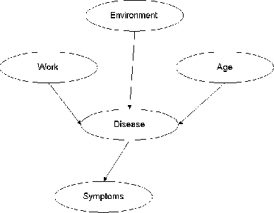
Figure 3.1: A Bayesian Network example.
In probability theory, P(A) denotes the probability that event A will occur. Belief measures in Bayesian formalism obeys the three basic axioms of probability theory:
![]()
![]()
If A and B are mutually exclusive, then:
![]()
The Bayes rule is the basis for Bayesian Networks:
![]()
Where ![]() is called the posterior probability and
P(H) is called the the prior probability.
is called the posterior probability and
P(H) is called the the prior probability.
Probability can be seen as a measure of belief in how probable outcomes are, given an event (subjective interpretation). It can also be interpreted as a frequency; how often it has happened in the past (objective interpretation).
When Bayesian Networks are applied in Data Mining, the user may want to apply techniques to learn the structure of a Bayesian network with one or more variables, or to reason on a structure that is already known.
With only one variable, the task is to compute a distribution for the
variable given any database. For instance, if we want to compute the
probability distribution for a coin that is flipped,
the distribution for the variable ![]() would be: ([7])
would be: ([7])
![]()
Where ![]() denote the background knowledge of the model, h denotes the
number of heads and t the number of tails.
This result is only dependent on the data in the database. In general,
for a variable that can have more outcomes, the distribution for the
set of physical probabilities of outcomes,
denote the background knowledge of the model, h denotes the
number of heads and t the number of tails.
This result is only dependent on the data in the database. In general,
for a variable that can have more outcomes, the distribution for the
set of physical probabilities of outcomes, ![]() will be:
will be:
![]()
Where ![]() is the number of times x = k in D, and c is a normalization
constant.
is the number of times x = k in D, and c is a normalization
constant.
If the structure of the network, ![]() , is known in advance, the aim of the
analysis is to compute the probabilities on the vertices from the database
D. If the database is complete, and the variables are discretized into
r different outcomes, the probabilities can be computed according to
the following formula:
, is known in advance, the aim of the
analysis is to compute the probabilities on the vertices from the database
D. If the database is complete, and the variables are discretized into
r different outcomes, the probabilities can be computed according to
the following formula:

To learn a structure, we want to generate candidate Bayesian Networks, and choose the structure that is best according to the database we have.
The probability distribution in equation  gives the
probability distribution for the next observation after looking in the
database:
To find a Bayesian Network B for a database D, we can use metrics
together with a search algorithm. The metrics approximate
equation  , and some of the metrics are:
Some search methods that exist are:
If data are missing in the database, it can either be filled in using the posterior distribution. Or we can use Gibbs sampling, which approximates the expectation of any function with respect to it's probability distribution. Another alternative is to use the expectation-maximization (EM)-algorithm which can be used to compute a score from the BIC-metric.
Missing data can be filled in using Gibbs sampling or the posterior distribution. The method is relatively resistant to noise.
In order to make the Bayesian network structure, it has to be learned from the database. It can also exist as prior knowledge.
The output from Bayesian Network algorithms is a graph, which is easy to interpret for humans.
There exist classifiers that perform in linear time, but further iterations give better results.
The method is statistically founded, and is always possible to examine why the bayesian method produced certain results.
Inductive Logic Programming (ILP) is a method for learning first-order definite clauses, or Horn clauses, from data. A Horn clause can be:
![]()
Where the predicate daughter is defined by the predicates female and parent. The two last predicates should be present as attributes in a relational schema in a database, and the new predicate daughter can be the result that has been learned.
The training examples that are used to learn a predicate p are
denoted ![]() . The ground facts which are known to belong to
the target relation are denoted
. The ground facts which are known to belong to
the target relation are denoted ![]() + and the facts that are
known not to belong to the target relation
+ and the facts that are
known not to belong to the target relation ![]() -. The ground
facts are taken from a database.
-. The ground
facts are taken from a database.
We use a concept description language ![]() to specify
syntactic restrictions on the definition of the predicates.
to specify
syntactic restrictions on the definition of the predicates.
To learn one or more predicates, we may also have background
knowledge, denoted ![]() and other predicates, denoted
and other predicates, denoted
![]() .
.
The quest is then to find a definition for a new predicate or set of
predicates, ![]() , expressed in
, expressed in ![]() such that
such that
![]() is complete (
is complete ( ![]() +) and consistent (
+) and consistent ( ![]() -) with respect to the training examples,
the background knowledge
-) with respect to the training examples,
the background knowledge ![]() and other predicates.
and other predicates.
A clause c is more general than clause d if c can be matched with
a subset of d. For instance, the clause ![]() is more general than
is more general than ![]() .
.
The least general generalization of two clauses ![]() and
and ![]() is the
least general clause which is more general than both
is the
least general clause which is more general than both ![]() and
and ![]() with
respect to the background knowledge
with
respect to the background knowledge ![]() .
.
ILP systems can be divided in three groups [6]: Empirical systems, which are single-predicate learning systems that are able to analyze large example sets with little or no human interaction. Interactive systems incrementally build complex domain theories consisting of multiple predicates where the user controls and initiates the model construction and refinement process. Programming assistants learn from small example sets without interaction with humans. The systems can use a multitude of techniques when inducing knowledge. The techniques are discussed briefly below. A more thorough discussion can be found in [2].
Inverse Resolution is motivated by the fact that in deduction, results found by resolution are clauses. We invert this procedure to find clauses from results.
The method uses the relative least general generalization (described in
section  ) to compute the most general clause given the background knowledge
![]() .
.
The top-down learner starts from the most general clause and repeatedly refine until it no longer covers negative examples. During the search the learner ensures that the clause considered covers at least one positive example.
A rule model is a rule on the form ![]() , where
T and
, where
T and ![]() are literal schemas. Literal schemas
are literal schemas. Literal schemas ![]() has
the form
has
the form ![]() or not
or not ![]() where all non-predicate variables
where all non-predicate variables ![]() are implicitly universally quantified.
are implicitly universally quantified.
All possible instantiations of the predicate variables are tried systematically for each rule model, and the resulting clauses are tested against the examples and background knowledge to produce new clauses that can be learned.
An ILP problem is transformed from relational to attribute-value form and solved by an attribute-value learner. This approach is only feasible for a small number of ILP problems where the clauses are typed, constrained and non-recursive. The induced hypothesis is transformed back into relational form.
Early ILP systems did not handle noise, but recent systems such as FOIL and LINUS are able to cope with noise.
General rules can not be generated from inconsistent data. Inconsistency must be removed by preprocessing the data.
The ILP methods require background knowledge on the form of definite clauses.
The output is given as definite clauses, often in Prolog syntax.
Inductive logic programming has a mathematical basis, and it is always possible to analyze why results are produced.
Overfitting can be a problem, if rules are generated that has low support.
The Rough Sets method was designed as a mathematical tool to deal with uncertainty in AI applications. Rough sets have in the last years also proven useful in Data Mining. The method was first introduced by Zdzislaw Pawlak in 1982 [11], the work have been continued by [18],[12], [17], [9] and others. This section is a short introduction to the theory of Rough Sets. A more comprehensive introduction can be found in [9] or [10].
The starting point of Rough Sets theory is an information
system, an ordered pair ![]() . U is a non empty
finite set called universe, A is a non empty finite set of
attributes. The elements
. U is a non empty
finite set called universe, A is a non empty finite set of
attributes. The elements ![]() of the universe
are called objects, and for each attribute
of the universe
are called objects, and for each attribute ![]() , a(x)
denotes the value of attribute a for object
, a(x)
denotes the value of attribute a for object ![]() . It is
often useful to illustrate an information system in a table, called an
information system table. One of the most important concepts in
Rough Sets is indiscernibility, denoted IND(). For an
information system
. It is
often useful to illustrate an information system in a table, called an
information system table. One of the most important concepts in
Rough Sets is indiscernibility, denoted IND(). For an
information system ![]() , an indiscernability
relation is:
, an indiscernability
relation is:
![]()
where ![]() . The interpretation of
. The interpretation of ![]() is that
the objects
is that
the objects ![]() and
and ![]() can not be separated by using the attributes in
the set B. The indiscernible objects can be classified in
equivalence classes:
can not be separated by using the attributes in
the set B. The indiscernible objects can be classified in
equivalence classes:
![]()
again ![]() .
. ![]() denotes an equivalence class based in
the attributes in set B. The set U/IND(B) is the set of all
equivalence classes in the relation IND(B). Intuitively the objects of
an equivalence class are indiscernible from all other objects in the
class, with respect to the attributes in the set B. In most cases we
therefore consider the equivalence classes and not the individual
objects. The discernibility matrix of an information system A,
with n attributes, is a symmetric
denotes an equivalence class based in
the attributes in set B. The set U/IND(B) is the set of all
equivalence classes in the relation IND(B). Intuitively the objects of
an equivalence class are indiscernible from all other objects in the
class, with respect to the attributes in the set B. In most cases we
therefore consider the equivalence classes and not the individual
objects. The discernibility matrix of an information system A,
with n attributes, is a symmetric ![]() matrix with
matrix with ![]() given by:
given by:
![]()
hence, ![]() contains the attributes upon witch classes
contains the attributes upon witch classes ![]() and
and
![]() differs.
differs.
Some of the objects attributes may be less important than
others when doing the classification. An attribute a is said
to be dispersible or superfluous in ![]() if IND(B)=IND(B-{a}) Otherwise the attribute is
indispensable in B. A minimal set of all the attributes that
preserves the partitioning of the universe is called a reduct,
RED. Thus a reduct is a set of attributes
if IND(B)=IND(B-{a}) Otherwise the attribute is
indispensable in B. A minimal set of all the attributes that
preserves the partitioning of the universe is called a reduct,
RED. Thus a reduct is a set of attributes ![]() such
that all attributes
such
that all attributes ![]() are dispensible and IND(B)=IND(A).
There are also object-related reducts that gives the set of
attributes needed to separate one particular object/class from all the
other.
are dispensible and IND(B)=IND(A).
There are also object-related reducts that gives the set of
attributes needed to separate one particular object/class from all the
other.
The theory is illustrated in the example below.
The next to define is the lower and upper approximation,
Rough definability of sets and the Rough membership
function. The lower and upper approximation are used to classify a
set of objects, X, from the universe that may belong to different
equivalence classes. Let ![]() and
and ![]() , the
B-lower,
, the
B-lower, ![]() and B-upper,
and B-upper, ![]() approximation
are:
approximation
are:
![]()
![]()
Hence this is a way to approximate X using only the attributes in the
set ![]() . The set
. The set ![]() is called
the boundary of X. Intuitively, the objects in
is called
the boundary of X. Intuitively, the objects in ![]() are the objects that are certain to belong to X, while the objects in
are the objects that are certain to belong to X, while the objects in
![]() are possible members of X, as illustrated in
Fig
are possible members of X, as illustrated in
Fig  .
.
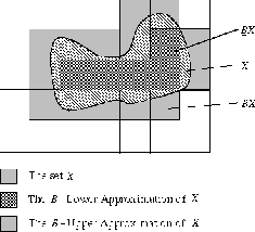
Figure 3.2: The B-upper and B-lower approximations of X.
If ![]() and
and ![]() then X is
said to be Roughly B-definable. If
then X is
said to be Roughly B-definable. If ![]() and
and ![]() then X is said to be Internally
B-undefinable. If
then X is said to be Internally
B-undefinable. If ![]() and
and ![]() then X is said to be Externally B-undefinable. If
then X is said to be Externally B-undefinable. If
![]() and
and ![]() then X is said to be
Totally B-undefinable
then X is said to be
Totally B-undefinable
The rough membership function ![]() , where
, where ![]() , is given by:
, is given by:
![]()
The rough membership function denotes the frequency of ![]() in X,
or the probability of X being a member of
in X,
or the probability of X being a member of ![]() .
.
A natural extension of the information system is the decision system.
A decision system is an information system with an extra set of
attributes, called decision attributes, hence
![]() . In most cases the set D has only one element,
. In most cases the set D has only one element,
![]() , and we will use this simplification in the rest of this
section. The decision attribute, d, reflects a decision made by
an expert. The value of d,
, and we will use this simplification in the rest of this
section. The decision attribute, d, reflects a decision made by
an expert. The value of d, ![]() is often a set of integers
{1,...,r(d)}, where r(d) denotes the range of d. It is also possible
to represent non numerical decisions, but then it is much simpler to
encode the decision into integers, e.g. false and true can be encoded
0 and 1 respectively. The partitioning
is often a set of integers
{1,...,r(d)}, where r(d) denotes the range of d. It is also possible
to represent non numerical decisions, but then it is much simpler to
encode the decision into integers, e.g. false and true can be encoded
0 and 1 respectively. The partitioning ![]() of the universe is denoted a decision class, and is a
classification of the objects in
of the universe is denoted a decision class, and is a
classification of the objects in ![]() determined by the
decision attribute d. A decision system is said to be
consistent
determined by the
decision attribute d. A decision system is said to be
consistent if for
all
![]()
Otherwise, the decision system is inconsistent . An inconsistent system is a system
where two or more of the objects have the same value for the set of
attributes A, hence belonging to the same equivalence class, but the
decision attribute d differs. A Decision table is a
table of the indiscernability classes, the attributes and the decision
attribute. The example below illustrates this.
When using rough sets as a algorithm for data mining, we generate
decision rules that map the value of an objects attribute to a
decision value. The rules are generated from a test set. If
![]() is a decision system, and a descriptor a=v,
where
is a decision system, and a descriptor a=v,
where ![]() , then a decision rule is
an expression generated from descriptor:
, then a decision rule is
an expression generated from descriptor:
![]()
Where ![]() ,
, ![]() are values of the attributes in A, d is the decision
attribute and v is the value of d. There are two types of decision
rules, definite and default decision
rules. Definite decision rules are rules that map the attribute
values of an object into exactly one decision class. A deterministic
decision system can be completely expressed by a set of definite
rules, but an indeterministic decision system can not.
are values of the attributes in A, d is the decision
attribute and v is the value of d. There are two types of decision
rules, definite and default decision
rules. Definite decision rules are rules that map the attribute
values of an object into exactly one decision class. A deterministic
decision system can be completely expressed by a set of definite
rules, but an indeterministic decision system can not.

To model an inconsistent decision system [9] suggests using a
set of rules called default rules.
Given a decision system ![]() and a threshold value
and a threshold value
![]() . A default rule for
. A default rule for
![]() with respect to the threshold is any decision rule
where:
with respect to the threshold is any decision rule
where:
![]()
Depending on the threshold value, it will be generated zero, one or more mutually inconsistent rules. A threshold of 1 gives only the set of default rules that are exactly identical to the set of definite rules. A threshold value greater than 0.5 maps the value of an objects attributes of an inconsistent equivalence class into only one decision class,where as a threshold value below 0.5 may map into several decision classes.
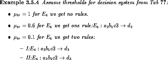
Definite and default rules generated directly from the training set, tends to be very specialized. This can be a problem when the rules are applied to unknown data, because many of the objects may fall outside, i.e. not match, of the specialized rules. If we make the rules more general, chances are that a greater number of the objects can be matched by one or more of the rules. One way to do this is to remove some of the attributes in the decision system, and by this glue together equivalence classes. This will certainly increase the inconsistency in the decision system, but by assuming that the attributes removed only discerns a few rare objects from a much larger decision class, this may not be a problem in most cases.

The subsections below compare the Rough Set method to the
criterias outlined in chapter  . This comparison will give us a
framework that can be used to compare the various data mining
techniques.
The rough set method is capable of handling most types of noise. If the input data is missing an attribute that is dispencible then the classification process is not affected. If the input data are missing important attributes, then the Rough Sets can not classify the object and the object must be thrown away. There are algorithms implemented that can 'guess' the value of a missing attribute, by doing statistical insertion among others, and thereby keeping the object.
Rough set method does not use prior knowledge when generating default rules. As mentioned before the default rules generated by Rough Set algorithms are generated only from the objects in the input data.
The output from the Rough Set algorithms are rules, preferably default
rules. These rules can then be uses to predict decisions based on the
input attributes. By making variations in the threshold value,
![]() one can tune the number of default rules to get the most
optional result. Rules are easy for humans to interpret and use.
one can tune the number of default rules to get the most
optional result. Rules are easy for humans to interpret and use.
The complexity of partitioning is O(nlog(n)), a sort algorithm. Computing the reducts is NP-complete, but there are approximation algorithms (genetic, Johnson, heuristical search) that have proven very efficient.
It is easy for the user to find out how the results were generated. This is because Rough Sets method can display the indiscernability classes it created and the distribution of the objects in these classes. The user can from this confirm the rules generated, and argument, in basis of the classes, why the rules are correct.
To experiment with the methods chosen, we selected the tools Rosetta, which is a Rough Set analysis tool and AutoClass, which is a Bayesian Networks classifier. The experiments were done on the OREDA database, which was supplied through the NOEMIE project.
OREDA is a reliability database for the oil industry, which has been in use for more than ten years. It contains data from ten different oil companies, and consists of three parts:
Most attributes in the database are composed of a number of codes which for instance describe types of failures. Text strings that can give further information are usually provided. There are several missing attribute values in the database.
The experiments was done on a 200MHz Pentium Pro processor running Windows NT 4.0. The OREDA database was stored in Oracle, and data retrieved using SQL*Plus 3.3.
AutoClass C version 3.0, compiled for MS-DOS, was used in testing. This is a public domain C-version of AutoClass III. Except where indicated, AutoClass searched for five minutes for classes. The Rosetta program used was a trial version 1.0b, limiting the decision system to 50 attributes and 5000 objects. Both programs had some minor bugs.
AutoClass is a tool for unsupervised classification using Bayesian methods to determine the optimal classes. AutoClass was developed at the NASA Ames Research Center. A description is given in [14].
In AutoClass, data must be represented in a data vector, with discrete nominal values or real scalar values. Each information vector is called a case, but we will still use the term object for each vector. The vectors can be stored in text- or binary files.
A class is a particular set of attribute (or parameter) values and their associated model. A model is either Single multinomial, Single normal or Multi normal. The first two models assume that attributes are conditionally independent, given a class; the probability that a class would have a particular value of any attribute depend only on the class and is independent of all other attribute values. The Multi normal model expresses mutual dependencies within the class.
Class membership is expressed probabilistically. The sum of probabilities for an object must always sum to one.
AutoClass has three options:
The Case number membership lists objects for each class with a
configurable number of attributes. It also lists the probability that
the object is put in each class. An example is given in Fig  .
.

Figure 4.1: An extract from a Case Number Membership cross reference.
Most probable class lists each object in the database, and lists
probabilities for which classes it is likely to be grouped in. An example
of a Most probable Class cross reference is given in Fig  .
.

Figure 4.2: An extract from a Most Probable Class cross reference.
The Class strength given in the Influence value report is a heuristic measure of how strongly each class predicts its instances.
The Normalized weight is a value between 0 and 1 that gives a probability value that a new object will be classified as a member of the given class.
Rosetta is a toolkit for pattern recognition and Data Mining, within the framework of Rough Sets. It is developed as an cooperative effort between the Knowledge System Group at NTNU, Norway and the Logic Group at the University of Warsaw, Poland. Further information on Rosetta can be found in [8].
Rosetta runs on Windows NT, and consists of a kernel and a Graphical User
Interface (GUI). The user interacts with the kernel through the GUI, but
the kernel is an independent unit. The GUI in Rosetta relies on human
interaction and human editing. Data are imported as a decision table
from a text file. The format of this text file is shown in Fig  .
.

Figure 4.3: Example of input file for Rosetta.
The first line contains the attribute names, the second contains the attribute types; integers, real numbers (float) or strings. Then the objects are listed successively. Missing attributes are denoted Undefined.
Rosetta organizes the data in a project and displays relations
between the various project items in project trees. Through
these trees the user can monitor and manually edit the steps in the
process. Most of the structure are displayed in tabular
form. Fig  is a screen shot from Rosetta, showing the
project tree to the left and a decision table to the right.
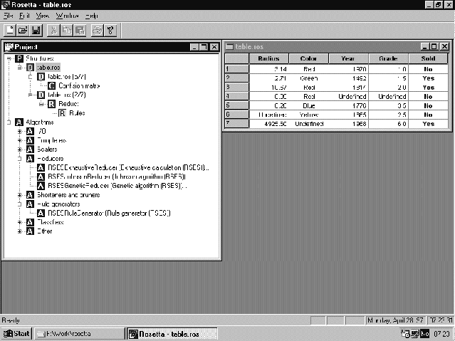
Figure 4.4: Screen shot from Rosetta.
Rosetta can handle missing attribute values by either removing the objects with missing values or inserting a mean value based on the value from the other objects attribute values. Other kind of preprocessing like splitting into test set and training set, manual removal of selected attributes and/or objects and discretizations are also supported. The user can calculate reducts, both normal and object oriented, and generate rules. The reducts can be calculated by three different algorithms; RSES exhaustive calculation, Johnson algorithm and genetic algorithm. All of the algorithms also supports dynamic calculation, which can be seen as combining normal reduct computation with statistical resampling techniques. Both the reducts and rules can be pruned away based on support value or with respect to a decision value or an attribute. It is also possible to calculate the rough classification for the decision system. The decision system and the rules can be exported as Prolog clauses.
Rosetta has also a possibility for testing the rules that have been
generated. The rules are applied on a test set with known decision
values. The result from the test is a confusion matrix, which is a
matrix where the predicted decisions values are compared to the actual
decision values, see Tab  for an example. The steps done
on the data are recorded together with the data, therefore reproduction
of the results are easy to do.

Table 4.1: An example of a confusion matrix.
We did three different experiments, with different data sets. The
presentation of their results from each experiment is split into two
parts, one for Rosetta results and one for the results from
AutoClass. We have tried to use tables and figures to show the
results. Comments and evaluation of the results are presented in
chapter  . An overview of values, with explanations of
selected attributes are included in appendix
  .
.
We extracted the datasets from the OREDA database using SQL. The SQL
statements are included in appendix  . We manually
preprocessed the data in MS-Notepad and through PERL scripts. This was
done to remove unwanted space between the attribute values, and to
insert attribute types and Undefined for missing values in the
Rosetta input file.
The model used in AutoClass in the experiments to follow was Single multinomial. All attributes were treated as discrete values. The reason for this is that AutoClass expects a zero-point and a relative error for scalars. By using discrete values, we were able to make the input more similar to the input to Rosetta. The datasets were preprocessed in Rosetta and the splits used in Rosetta were exported using cut and pasted into MS-Notepad.
We manually read the database diagrams and chose the attributes that we
thought had some possible functional dependencies. The attributes,
with explanation are listed in Tab  .
.

Table 4.2: Table of the attributes in Experiment I.
When we manually inspected the data we found that the values in
attributes I_MANUFACT_CTRL_SYS and I_SUBSEA_CS were
mostly missing, so we removed them. We also removed three objects out of
3357 that had most of the attribute values missing. Tab  below
shows the number of objects and attributes in the dataset of experiment I.
![]()
Table 4.3: Facts on Experiment I data set.
The dataset was randomly split into a 30% training set, and a 70% test set.
We wanted to see if it was possible to predict the failure type given the values from the other attributes. We chose the attribute FM_CODE as decision attribute. Then we calculated dynamic reducts, both normal and object oriented, and generated rules. We tested the rules on the test set, and the overall hit rate was around 59%. We then tried to remove four of the attributes that had missing attributes, but this did not improve the results.
After 62 tries, AutoClass found nine classes. The strength of each class is
given in Tab  , and the influence of each attribute is given in
Tab
  .
.
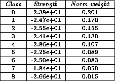
Table 4.4: Strength and normalized weight for the classes in Experiment I.
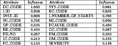
Table 4.5: The relative influence of each attribute in Experiment I.
To get more background information we contacted an expert on the OREDA
database. He suggested that we restricted the dataset to faults on
one type of equipment. We selected Gas Turbines because it had
many reported failures, and Electro Motors because it had few
reported failures. In this way we could test the tools on a set with
many objects and on a different set with fewer objects. We selected a
new set of attributes, which are listed in Tab  . The facts
about the Gas Turbines dataset and Electro Motors dataset
is shown in Tab
  . The Electro Motors set was randomly split
into a 30% training set and a 70% test set. The Gas Turbines set was
randomly split in two different sets for training and testing, with
the percentage for training set and test set respectively, 20-80% and
30-70%.
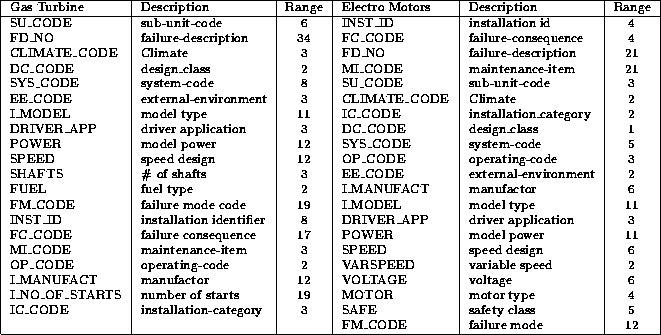
Table 4.6: Table of the attributes in Experiment II.

Table 4.7: Facts on Experiment II data set.
We kept FM_CODE as the decision attribute calculated the
dynamic reducts for the training set, and generated rules. We then
created the confusion matrix, but the overall results was only 19%.
We then tried to remove the missing attribute values in the decision
table by applying mean/mode fill. This removed the incompleteness, but
the rules we got now did not give us any better results. The overall
performance for all the tests are recorded in Tab  .
.

Table 4.8: The results from the Electro Motor test.
We kept FM_CODE as decision attribute, and did five different tests. These were:
 .
.
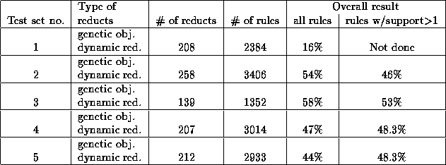
Table 4.9: The results from Gas Turbine test.
Experiments with the Gas Turbine set was not done in AutoClass.
After 2087 tries, AutoClass found four classes. The strength
of each class is given in Tab  , and the influence of each attribute
is given in Tab
  .
.
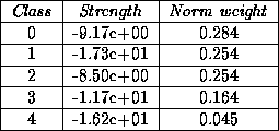
Table 4.10: Strength and normalized weight for the classes in the Electro Motor dataset.
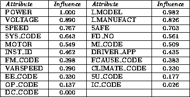
Table 4.11: The relative influence of each attribute in the Electro Motor dataset.
We tried running tests on a decision attribute with a
smaller range. We selected SEVERITY as the new decision
attribute. It has four different values, Critical - C,
Degraded - D, Incipient - I and Unknown - U,
hereas FM_CODE has a range of 42 different values. The goal
of our search has now changed from finding the failure type to predict
the severity of the failures, given certain attributes.
This time we only worked with the Gas Turbine set. The attributes we used also
reduced from 21 to 14, see Tab  .
.
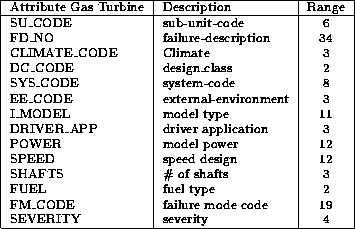
Table 4.12: Table of the attributes in Experiment III.
The attributes removed were either attributes where the value was
equal, or missing, in most objects, f.x. IC_CODE, or the value
had little or no information, f.x. FCAUSE, or the value where
implicitly given by other values, f.x. I_MANUFACT. We noticed
that the value U was only used in six out of 1198 objects, so
we removed those objects to reduce the range of SEVERITY. The
distribution of SEVERITY is listed in Tab 

Table 4.13: The distribution of Severity.
The gas turbine set was randomly split into three different sets of
test/training set, with the percentage for training set and test set
20-80%, 30-70% and 50-50%, respectively. Facts about the set are
shown in Tab 
![]()
Table 4.14: Facts on Experiment III data set.
This time we did three different tests one for each of the splitting
types. The results before pruning are shown i Tab 

Table 4.15: Results from Experiment III-a.
We decided to do the pruning more carefully to try to discover how
many rules was needed to make good predictions. In Fig  we have
plotted the overall results versus the support, for all of the three
test sets, and in Tab
  we have listed the number of rules
left after pruning away the rules with support less than 2, 5, 10, 25,
40 and 50.

Table 4.21: Number of rules left after pruning w.r.t. support.
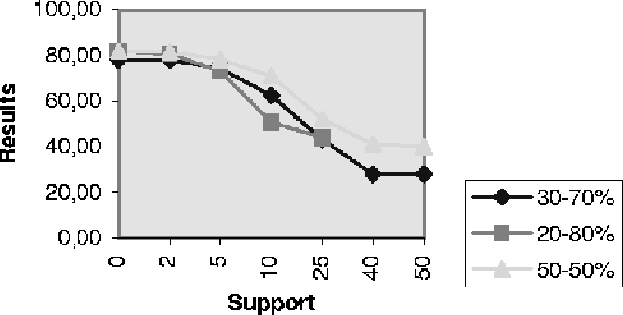
Figure 4.5: Overall result versus the support for Experiment III-a.
Tab  , Tab
, Tab  and Tab
  contains
examples of the strongest reducts, e.g. the reducts with the greatest
support, the strongest rules and an example of a confusion matrix.
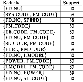
Table 4.17: Example of strong reducts.

Table 4.18: Example of strong rules.

Table 4.19: Example of confusion matrix.
The confusion matrixes in Tab  shows that the decision C is
well predicted, but the decisions D and I are more
difficult to distinguish. This can be a problem if we want
to identify every severity type. But if we want to distinguish the
critical failures from the non-critical it is possible to group
D and I into one decision value O. This leaves 378
objects with decision C and 819 objects with decision O
We tried this, and the results are presented in Tab
  .
.
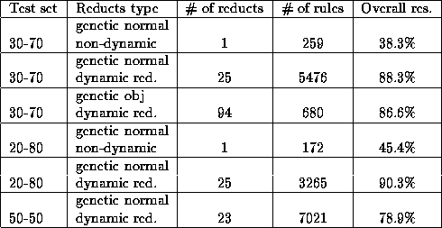
Table 4.20: Results from Experiment III-b.
Pruning was done on the rules generated from the normal dynamic
reducts, and are plotted in Fig  , listed in
Tab
  , in the same way as for the previous experiment. We
also have examples of reducts, rules and confusion matrixes, they are
in Tab
  , Tab
, Tab  and Tab
  ,
respectively.

Table: Number of rules left after pruning w.r.t. support.
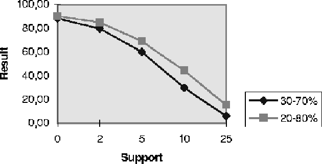
Figure 4.6: Overall result versus the support for Experiment III-b.

Table 4.22: Examples of strong reducts.

Table 4.23: Examples of strong rules.

Table 4.24: Example of a confusion matrix.
Experiments were conducted on 20%, 30% and 50% of the data as training set. Finally, the range of the decision attribute in Rosetta was reduced, and the experiment ran in AutoClass as well to see if it had any influence on the classes generated.
After 541 tries, AutoClass found nine classes.
The strength of each class is given in Tab  , and the influence of
each attribute is given in Tab
  .
.
The classes were manually inspected, and identified after the name of the manufacturer. A description of each class is listed below:
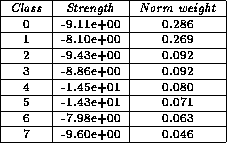
Table 4.25: Strength and normalized weight for the classes in the Gas Turbine set with 20% training set.
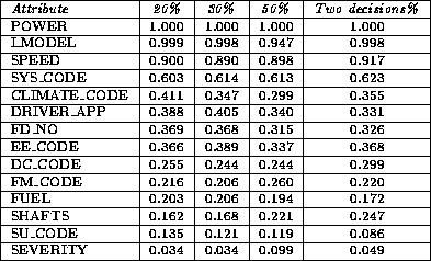
Table 4.26: The relative influence of each attribute for the different training sets.
After 246 tries, AutoClass found seven classes. The strength of each class is given in
Tab  , and the influence of each attribute is given in Tab
  .
We also tried to let AutoClass search for classes for five hours on the set, but
this did not change the result.
The classes generated were:
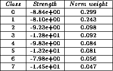
Table 4.27: Strength and normalized weight for the classes in the Gas Turbine set, 30% training set.
After 139 tries, AutoClass found twelve classes. The strength
of each class is given in Tab  , and the influence of each attribute
is given in Tab
  .
.
The classes generated were:
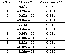
Table 4.28: Strength and normalized weight for the classes in the Gas Turbine set, 50% training set.
After 252 tries, AutoClass found nine classes. The strength
of each class is given in Tab  , and the influence of each attribute
is given in Tab
  . The training set was 30%.
The classes generated were:
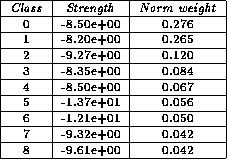
Table 4.29: Strength and normalized weight for the classes in the Gas Turbine set, two decisions.
In this chapter, we discuss the results from the experiments described
in chapter  . We will first evaluate results from Rosetta,
then from AutoClass, and finally we compare the results with respect to
the NOEMIE project.
The results obtained from Rosetta was only partly good. The first two experiments had rather low overall results, especially experiment II. Reasons for the low results in experiment I may be a combination of wrong attributes, missing attribute values and a too large range of the decision value. The electro motor part of experiment II suffered from too many missing attribute values. When they were removed we were left with to few objects to get a good classification. In the gas turbine part, the same problems as in experiment I occurred.
Experiment III gave a much better overall result than the two previous
ones. It may therefore be interesting to examine some of the reducts
and rules generated here, in greater detail. The reducts are presented
in Tab  and in Tab
  . The first observation to
make is that the reducts are short, only one or two attributes in
experiment III-a, three decisions, and two to four in experiment
III-b, two decisions. This indicates that decisions can be drawn based
on just a few attributes. We also notice that the attributes
FM_MODE and FD_NO are present, either alone or
together in all of the reducts. This makes sense, since
SEVERITY ought to depend on the failure type and description.
When we look at the rules in Tab  and Tab
  ,
we first notice that there are many. They also generally have low support.
This is not an advantage, because then the
rules are somewhat specialized. When the weaker rules, the most
special, were pruned away, the overall results were dropping. This
is illustrated in Fig
  and Fig
  . We see that
the rules with the lowest support (<2) can be removed without
loosing classification power. This halves the number of rules. If we
remove more rules, the one with support<5, we reduce the the rule
set with approximately another 60%, but we also increase the number
of unclassified objects. There is a trade off between few, strong rules
and many unclassified objects. But the quality of some of the
strongest rules are high. In Tab
  the second and third
rule are short and general. This is because, due to rules in the OREDA
database, the SEVERITY of a failure of type AIR,
FM_MODE(AIR) is always Incipient (I), and the
SEVERITY of a failure of type FTS, FM_MODE(FTS)
is always Critical (C). Rosetta had not this background
information, and it showed strength by finding these dependencies.
Below are some of the indications that we think can be drawn on Rosetta used on the OREDA database based on the results we have obtained.
The number of attributes is not as important as to what attributes to include. Irrelevant attributes can in some cases confuse Rosetta, but in most of the experiments Rosetta used only the most important attributes, and discarded the rest, in the reducts. We also found that there is a relationship between the number of attributes, their range, and the number of objects needed to make good rules. Thus, if we have many attributes, we must have more objects than with fewer attributes, to generate good rules.
We found that in most cases the rules from Rosetta gave us an overfit problem, there were too many specialized rules. This problem could be corrected by applying pruning. We saw some indications, especially in experiment III that the degree of overfit increased with increasing size of the training set.
We saw for experiment II and III, that the range of decision values is important to the overall result. It is difficult for Rosetta to make classification on too many different decisions. But, again, this depends much on the dataset.
We did not do tests that could indicate runtime complexity, nor did we do a comparison on the results versus time used on calculation. But we found that the time used for calculating reducts varied for the type of reduct. Dynamic reducts are much more computer intensive than normal reducts, and object-related reducts are more computer intensive than normal related. Calculating the dynamic reducts took from 10 to 40 minutes. Normal reducts was calculated within few minutes, sometimes less than one minute.
AutoClass classifies the data into classes that seems logical for humans. In Experiment II, the relative influence in classifying objects is highest for the attribute POWER. However, it is easy to interpret the classes after the attribute with the second highest influence, the model. The equipment units having I_MODEL = 1535-121G and Avnon1525-121G are grouped together. The units are probably the same, but have been given two labels in OREDA.
We observe that GT35B-850 and KG5 are always grouped together. Both are of design class "industrial" (DC_CODE = IN), as are the TORNADO units, which are grouped together with the two when the training set is 20%.
The attribute with the highest relative influence in experiment I was the DESIGN CLASS attribute, which is what we would expect that a human would use to discern between the data.
Some indications that can be drawn from the experiments with AutoClass on OREDA are listed below:
We varied the number of attributes in the experiments from 14 to 21. The number of classes found were between four and eleven. Experiment I with 18 attribute values produced eight classes, while experiment II with 21 attributes generated between eight and eleven classes when experiments was done on different training set sizes. Experiment III generated four classes, from a dataset with 14 attributes. It seems that the number of attributes have little influence on the number of classes produced.
The classes generated by AutoClass are described below for the different training set sizes:
It seems like more data leads to a more precise classification. We could expect that an unsupervised classifier would give an overfit classification for a small data size, but the number of classes are less (8) when the training set is 20% than when it is 50% (11).
AutoClass produced seven classes for the Gas Turbine set with a 30% training set. When the range for SEVERITY was reduced from three to two attribute values, eight classes was produces. Both had two classes with high relative normal weight (over 0.25), and the rest had low relative normal weight (less than 0.12). The relative influence of SEVERITY increased from 0.034 to 0.049. Class 4 was split into two classes of equal size, Class 7 and Class 8. Class 7 contained objects having POWER=9250 and I_MODEL=1304-10, and Class 8 had objects containing POWER=6900 and I_MODEL = TORNADO. We were not able to discover any pattern in the SEVERITY attribute (it was distributed equally in the classes).
The new classification may have occurred because the datasets are slightly different in the two experiments. The whole data set was split into test- and training set with different random seeds, but this can probably not explain the split of the classes.
AutoClass did not produce any different results when we increased the search time from five minutes to five hours. We did not investigate further how much time AutoClass should search to find sufficiently good classes.
Rosetta and AutoClass differs in both appearance and underlying theory.
The tools and methods are discussed in the context of the NOEMIE
project. The comparisons follows most of the criterias outlined in
chapter  .
.
Neither of the tools are robust (they are not commercial products). AutoClass crashed when trying to produce reports after analyzing certain data sets, while Rosetta crashed after some series of operations.
The output from Rosetta is rules, whereas AutoClass returns classes. The rules generated by Rosetta and the classes that AutoClass finds can have several usages in NOEMIE. Rules generated can be used to:
The AutoClass output requires interpretation, and is not usable in the current form except for human analysis.
Rosetta has a way of testing how good the rules generated are on a test set, while AutoClass does not have a decision to test against and is only using the model it has learned to classify the test set.
Both methods are able to handle noise, but only as a normal attribute values. Neither of the methods handles attribute values that are ``not applicable''. The user must be cautious when trying to fill in values for missing and ``not applicable'' attribute values, because this can create unreliable results.
As a logical and statistical method, both are retractable, it is possible to find out how the tools discovered the rules or classes.
This chapter contains conclusions based on the theoretical descriptions of methods, experiments and the discussion. We also outline possible further work.
From the discussion in chaper  , the following conclusions
can be drawn after using Rosetta on the OREDA dataset:
For AutoClass, we can draw these conclusions after using it on OREDA:
Both tools can be used in the NOEMIE project, but for different purposes: AutoClass gives an understanding of the data by grouping them into classes, while the output of Rosetta can be used directly, as background knowledge in Case-Based Reasoning, and in making predictions about failures.
A central issue in the NOEMIE project will be to integrate the results from Data Mining with Case-Based Reasoning [3].
A case is defined as a previously experienced situation, and it is usually a problem situation with an interpretation and possibly annotations. Case-Based Reasoning methods identify a problem, and tries to find past cases that are similar to the new one. Then the old cases are used to suggest a solution for the new problem. The solution is evaluated, and the systems knowledge-base is updated with the new experience.
Questions that will have to be investigated further, are how the the results from the Data Mining process are to be collected for use in Case-Based Reasoning. The system should be able to handle uncertain data. It could also use metadata to decide what information to include when constructing cases.
After having carried out the experiments in chapter  , we
see several topics that would be interesting to investigate further:
Data mining (DM) eller Knowledge Discovery in Databases (KDD) som det ogsĺ blir kalt, inneholder mange teknikker og verktřy for ĺ finne informasjon i store datamengder. Metoden er en utvidelse av data analyse metoder for ĺ finne sammenhenger med flere relasjoner. Noen av disse teknikkene er inductive learning, pattern identification, concept discovery, statistical cluster og bayesian nettworks. Oppgaven gĺr ut pĺ ĺ evaluere noen av teknikkene som blir brukt og verktřy knyttet til disse. Spesielt vil du se pĺ verktřy som er utviklet i europeiske prosjekter (f. eks. INRECA, SODAS, STARS). Oppgaven er en del av et střrre EU-prosjekt med Sintef Tele og data, Sintef Sikkerhet og pĺlitelighet i tillegg til partnere fra Frankrike og Italia. Du vil jobbe nćrt knyttet til prosjektets deltakere, delta i det videre arbeidet i prosjektet, og du vil kunne fortsette med diplomoppgave.
Mĺl: Evaluere verktřy og teknikker.
Below, we list the definitions we used for some of the terms in the field of Data Mining and Knowledge Discovery.
Below is a list of the resources on the Internet we encountered during the work on this project.
Below, we list the SQL queries we used to get the data sets from the OREDA data base.
select failure_event.ec_code, failure_event.su_code, fcause_no,
sc_code, fd_no, fc_code, om_code, failure_event.inst_id,
failure_event.i_id,mi_code, ic_code, oc_code, climate_code, dc_code,
sys_code, op_code, ee_code, i_manufact, i_model, i_manufact_ctrl_sys,
i_no_of_starts, i_subsea_cs, fm_code

from failure_event,failure_item, inventory, installation

where failure_event.i_id=inventory.i_id AND
failure_event.owner_id=inventory.owner_id AND
failure_event.inst_id=inventory.inst_id AND
failure_event.f_id=failure_item.f_id AND
failure_event.owner_id=failure_item.owner_id AND
failure_event.inst_id=failure_item.inst_id AND
failure_event.owner_id=installation.owner_id AND
failure_event.inst_id=installation.inst_id ;
% SQL for Electric Motors

select fe.inst_id, fcause_no, fd_no, mi_code, fi.su_code, mi_code,
climate_code, ic_code, dc_code, sys_code, op_code, ee_code,
i_manufact, i_model, T.inv_spec_char Driver_App, T2.inv_spec_char
Power, T3.inv_spec_char Speed, T4.inv_spec_char Varspeed,
T5.inv_spec_char Voltage, T6.inv_spec_char Motor, T7.inv_spec_char
Safe, fm_code

from failure_event fe, failure_item fi, installation ins, inventory
iv, inv_spec T,inv_spec T2, inv_spec T3,inv_spec T4,inv_spec T5,
inv_spec T6, inv_spec T7

where fe.i_id=iv.i_id and iv.i_id=T.i_id and T.i_id=T2.i_id and
T2.i_id=T3.i_id and T3.i_id=T4.i_id and T4.i_id=T5.i_id and
T5.i_id=T6.i_id and T6.i_id=T7.i_id and fe.inst_id=iv.inst_id and
iv.inst_id=ins.inst_id and ins.inst_id=fi.inst_id and
fi.inst_id=T.inst_id and T.inst_id=T2.inst_id and
T2.inst_id=T3.inst_id and T3.inst_id=T4.inst_id and
T4.inst_id=T5.inst_id and T5.inst_id=T6.inst_id and
T6.inst_id=T7.inst_id and T.attr_field='APPLIC1' and
T2.attr_field='POWER' and T3.attr_field='SPEED' and
T4.attr_field='VAR_SPEED' and T5.attr_field='VOLTAGE' and
T6.attr_field ='TYPE3' and T7.attr_field='SAFECLS' and fe.f_id=fi.f_id

% SQL for Gas Turbines

select fe.inst_id, fcause_no, fd_no, mi_code, fi.su_code, mi_code,
climate_code, ic_code, dc_code, sys_code, op_code, ee_code,
i_manufact, i_model, i_no_of_starts, T.inv_spec_char Driver_app,
T2.inv_spec_char Power, T3.inv_spec_char Speed, T4.inv_spec_char
Shafts, T5.inv_spec_char Fuel, fm_code

from failure_event fe, failure_item fi, installation ins, inventory
iv, inv_spec T,inv_spec T2, inv_spec T3,inv_spec T4,inv_spec T5

where fe.i_id=iv.i_id and iv.i_id=T.i_id and T.i_id=T2.i_id and
T2.i_id=T3.i_id and T3.i_id=T4.i_id and T4.i_id=T5.i_id and
fe.inst_id=iv.inst_id and iv.inst_id=ins.inst_id and
ins.inst_id=fi.inst_id and fi.inst_id=T.inst_id and
T.inst_id=T2.inst_id and T2.inst_id=T3.inst_id and
T3.inst_id=T4.inst_id and T4.inst_id=T5.inst_id and
T.attr_field='APPLIC1' and T2.attr_field='POWER' and
T3.attr_field='SPEED' and T4.attr_field='NUMBSHAFT' and
T5.attr_field='FUEL' and fe.f_id=fi.f_id
% SQL for Gas Turbines - severity as decition

select fe.inst_id, fcause_no, fd_no, mi_code, fi.su_code, mi_code,
climate_code, ic_code, dc_code, sys_code, op_code, ee_code,
i_manufact, i_model, i_no_of_starts, T.inv_spec_char Driver_app,
T2.inv_spec_char Power, T3.inv_spec_char Speed, T4.inv_spec_char
Shafts, T5.inv_spec_char Fuel, fm_code, sc_code

from failure_event fe, failure_item fi, installation ins, inventory
iv, inv_spec T,inv_spec T2, inv_spec T3,inv_spec T4,inv_spec T5

where fe.i_id=iv.i_id and iv.i_id=T.i_id and T.i_id=T2.i_id and
T2.i_id=T3.i_id and T3.i_id=T4.i_id and T4.i_id=T5.i_id and
fe.inst_id=iv.inst_id and iv.inst_id=ins.inst_id and
ins.inst_id=fi.inst_id and fi.inst_id=T.inst_id and
T.inst_id=T2.inst_id and T2.inst_id=T3.inst_id and
T3.inst_id=T4.inst_id and T4.inst_id=T5.inst_id and
T.attr_field='APPLIC1' and T2.attr_field='POWER' and
T3.attr_field='SPEED' and T4.attr_field='NUMBSHAFT' and
T5.attr_field='FUEL' and fe.f_id=fi.f_id
This appendix explains the codes used in some of the attribute values.

Table E.1: Description of the value codes for attribute Design
Class, DC_CODE, which is a classification based on the design of an item.

Table E.2: Description of the value codes for attribute
External Environment, EE_CODE, which is the
local environment where the item is placed.
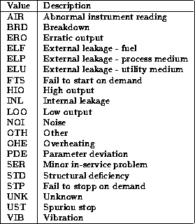
Table E.4: Description of the value codes for attribute Failure
Mode, FM_CODE, which describes the type of failure that has
occured.