Bayesian Networks

Bayesian networks is a statistical method for Data Mining, a statistical method for discovering valid, novel and potentially useful patterns in data. A description of Probabilistic networks and machine learning techniques is given in [15].

Bayesian networks are used to represent essential information in databases in a network structure. The network consists of edges and vertices, where the vertices are events and the edges relations between events. A simple Bayesian network is illustrated in Fig 3.2, where symptoms are dependent on a disease, and a disease is dependent on age, work and work environment. Introductions to Bayesian networks can be found in [13], [25], [17], [14] and [18].

Bayesian networks are easy to interpret for humans, and are able to store causal relationships , that is, relations between causes and effects. The networks can be used to represent domain knowledge, and it is possible to control inference and produce explanations on a network.

  

Figure 3.3: A Naive Bayesian Network.

A simple usage of Bayesian networks is denoted naive Bayesian classification [15]. These networks consist only of one parent and several child nodes as in Fig 3.3. Classification is done by considering the parent node to be a hidden variable (H in the figure) stating which class (child node) each object in the database should belong to. An existing system using naive Bayesian classification is AutoClass [29].

The theoretical foundation for Bayesian networks is Bayes rule, which states:

$$P(H \mid e) = \frac{P(e \mid H)P(H)}{P(e)}$$

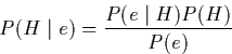
Where H is a hypothesis, and e an event. $P(e \mid H)$ is the posterior probability, and P(H) is the prior probability. A proof of Bayes rule is given in appendix A.

To give a formal definition of Bayesian networks, we introduce some terminology which is taken from [25]:

If a subset of Z nodes in a graph G intercepts all paths between the nodes X and Y (written $\langle X\mid Y\mid Z \rangle_G$), then this corresponds to conditional independence between X and Y given Z:

$$\langle X\mid Y\mid Z \rangle_G \Rightarrow I(X,Z,Y)_M$$

conversely:

$$I(X,Z,Y)_M \Rightarrow \langle X\mid Y\mid Z \rangle_G$$

with respect to some dependency model M.

 

Figure 3.4: X is Independent of Y Given Z.

A Directed, Acyclic Graph (DAG) D is said to be a I-map of a dependency model M if for every three disjoint sets of vertices, X, Y and Z we have:

$$\langle X\mid Y\mid Z \rangle_G \Rightarrow I(X,Z,Y)_M$$

A DAG is a minimal I-map of M if none of its arrows can be deleted without destroying its I-mapness.

Given a probability distribution P on a set of variables U, a DAG $D=(U,\vec{E})$ is called a Bayesian Network of P iff D is a minimal I-map of P.

A Bayesian network is shown in Fig 3.3, representing the probability distribution P:

$$P(x_6 \mid x_5)P(x_5 \mid x_2,x_3)P(x_4 \mid x_2,x_1)P(x_3 \mid x_1)P(x_2 \mid x_1) P(x_1)$$

  

Figure 3.5: A Bayesian Network Representing the Distribution P.